class: title-slide, middle, right .title-text[Mapping in R] .title-sub[1: making static maps in R with ggplot2] .title-spacer[] .title-presenter[Matt Kerlogue] .title-date[29 November 2019] --- # The data we'll be using .pull-left[ We'll be using the Cabinet Office's [Civil Service Statistics 2019](https://www.gov.uk/government/statistics/civil-service-statistics-2019). Specifically, the [machine readable](https://www.gov.uk/government/uploads/system/uploads/attachment_data/file/836368/Statistical-tables-Civil-Service-Statistics-2019-machine-readable-headcounts-version-V2.csv/preview) csv. ```r # download the civil service statistics data civil_service_stats_2019 <- readr::read_csv( "https://assets.publishing.service.gov.uk/ government/uploads/system/uploads/ attachment_data/file/836368/Statistical- tables-Civil-Service-Statistics-2019- machine-readable-headcounts-version-V2.csv", col_types = paste0(rep("c", 12), collapse ="")) ``` ] .pull-right[ 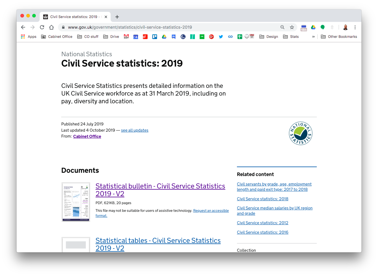 ] --- # ONS Geoportal .pull-left[ The ONS Geoportal (https://geoportal.statistics.gov.uk/), provides an extensive array of geographical information for mapping statistical outputs. Including: * **boundaries** - the shapes of geographical areas * **centroids** - point-based geographical data (including population weighted centroids) * **lookups** - tables to convert from one geography to another ] .pull-right[ 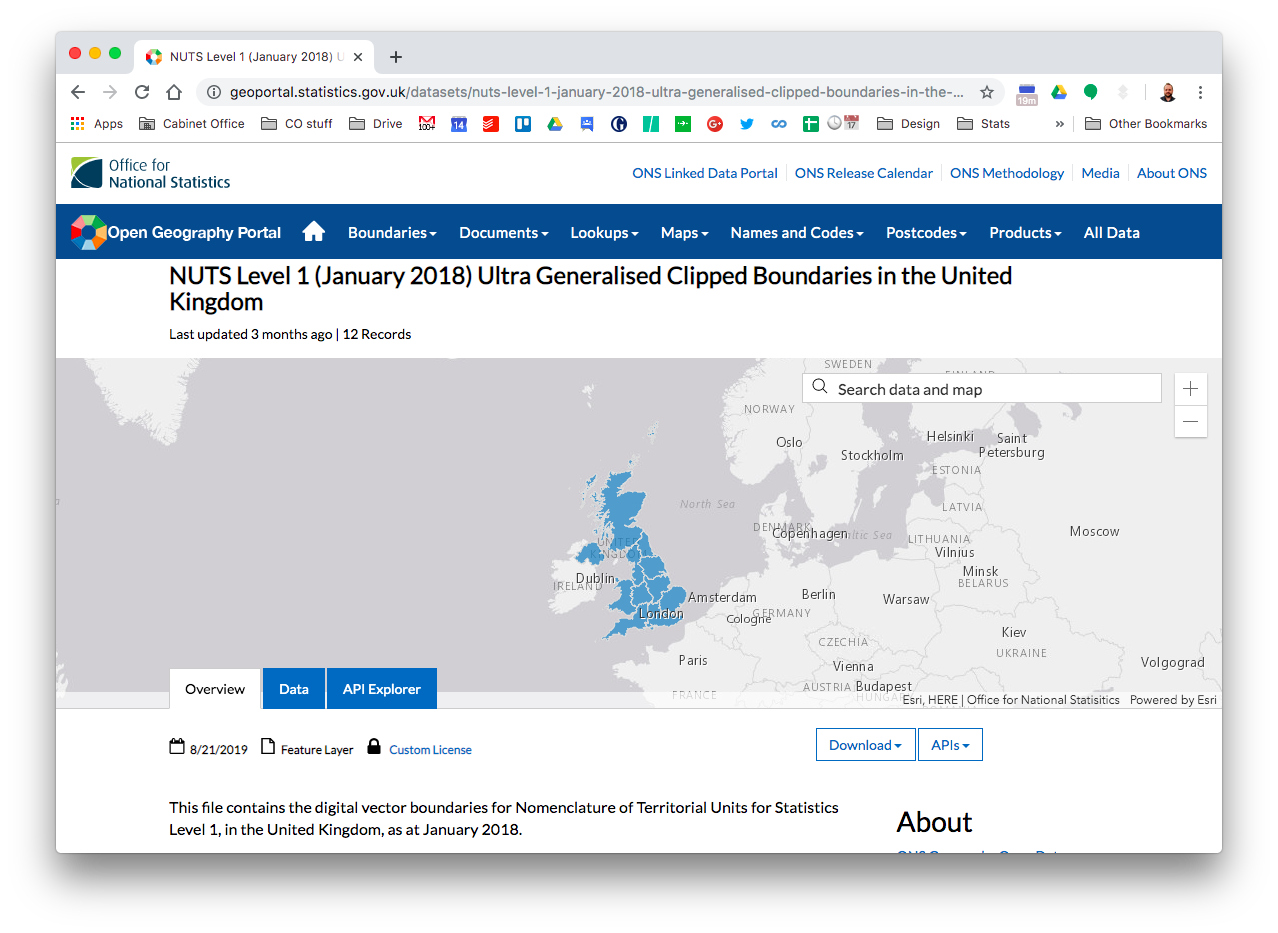 ] ---  --- .pull-left[ ```r t13_dt <- civil_service_stats_2019 %>% filter(table == "t13", category_2 == "All employees", category_4 == "Total") %>% mutate(value = as.numeric(value)) %>% group_by(category_1) %>% summarise(total = sum(value, na.rm = TRUE)) ``` * Filter to table T13 * Filter to the total number of all employees (by region) * Convert to numeric * Group by region (`category_1`) * Sum the totals ] -- .pull-right[ ``` ## # A tibble: 6 x 12 ## source table category_1 category_2 category_3 category_4 category_name_1 ## <chr> <chr> <chr> <chr> <chr> <chr> <chr> ## 1 Still… t13 East Permanent Female Full-time css_region_name ## 2 Still… t13 East Permanent Female Part time css_region_name ## 3 Still… t13 East Permanent Female Unknown css_region_name ## 4 Still… t13 East Permanent Male Full time css_region_name ## 5 Still… t13 East Permanent Male Part time css_region_name ## 6 Still… t13 East Permanent Male Unknown css_region_name ## # … with 5 more variables: category_name_2 <chr>, category_name_3 <chr>, ## # category_name_4 <chr>, measure <chr>, value <chr> ``` ``` ## # A tibble: 15 x 2 ## category_1 total ## <chr> <dbl> ## 1 All employees 445480 ## 2 East 21420 ## 3 East Midlands 19910 ## 4 London 89110 ## 5 North East 29400 ## 6 North West 54900 ## 7 Northern Ireland 3690 ## 8 Not reported 3060 ## 9 Overseas 4860 ## 10 Scotland 43930 ## 11 South East 38610 ## 12 South West 40240 ## 13 Wales 34110 ## 14 West Midlands 28180 ## 15 Yorkshire and The Humber 34090 ``` ] --- .pull-left[ ```r t13_dt <- civil_service_stats_2019 %>% filter(table == "t13", category_2 == "All employees", category_4 == "Total") %>% mutate(value = as.numeric(value)) %>% group_by(category_1) %>% summarise(total = sum(value, na.rm = TRUE)) %>% * filter(category_1 != "All employees", * category_1 != "Not reported", * category_1 != "Overseas") %>% * rename(region = category_1) ``` * Filter out the line for all employees, those for which there is no location, and those based overseas * Rename `category_1` to something useful ] -- .pull-right[ ``` ## # A tibble: 12 x 2 ## region total ## <chr> <dbl> ## 1 East 21420 ## 2 East Midlands 19910 ## 3 London 89110 ## 4 North East 29400 ## 5 North West 54900 ## 6 Northern Ireland 3690 ## 7 Scotland 43930 ## 8 South East 38610 ## 9 South West 40240 ## 10 Wales 34110 ## 11 West Midlands 28180 ## 12 Yorkshire and The Humber 34090 ``` ] --- # Back to geography.. .pull-left[ Region names are "ok"... but often different folk have different ways of naming and labelling geographic entities: "Yorkshire" / "Yorkshire and the Humber" / "Yorkshire and Humberside" / "Yorks and Humber". Let's download the UK region boundaries and see what the region names are: ```r sfdt <- st_read( "https://opendata.arcgis.com/datasets/ 01fd6b2d7600446d8af768005992f76a_4.geojson") ``` ] -- .pull-right[ ``` ## # A tibble: 12 x 5 ## objectid nuts118cd nuts118nm long lat ## <int> <fct> <fct> <dbl> <dbl> ## 1 1 UKC North East (England) -1.73 55.3 ## 2 2 UKD North West (England) -2.77 54.4 ## 3 3 UKE Yorkshire and The Humber -1.29 53.9 ## 4 4 UKF East Midlands (England) -0.850 52.8 ## 5 7 UKI London -0.309 51.5 ## 6 5 UKG West Midlands (England) -2.20 52.6 ## 7 6 UKH East of England 0.504 52.2 ## 8 8 UKJ South East (England) -0.993 51.5 ## 9 9 UKK South West (England) -3.63 50.8 ## 10 10 UKL Wales -3.99 52.1 ## 11 11 UKM Scotland -3.97 56.2 ## 12 12 UKN Northern Ireland -6.85 54.6 ``` ] --- .pull-left[ ``` ## # A tibble: 12 x 1 ## region ## <chr> ## 1 East ## 2 East Midlands ## 3 London ## 4 North East ## 5 North West ## 6 Northern Ireland ## 7 Scotland ## 8 South East ## 9 South West ## 10 Wales ## 11 West Midlands ## 12 Yorkshire and The Humber ``` ] .pull-right[ ``` ## # A tibble: 12 x 1 ## nuts118nm ## <fct> ## 1 North East (England) ## 2 North West (England) ## 3 Yorkshire and The Humber ## 4 East Midlands (England) ## 5 London ## 6 West Midlands (England) ## 7 East of England ## 8 South East (England) ## 9 South West (England) ## 10 Wales ## 11 Scotland ## 12 Northern Ireland ``` ] --- .pull-right[ There are many packages that enable R to handle spatial data. `{sp}`, `{rgdal}`, `{rgeos}` are the most common, but there are over 97 packages containing 'geo' in their name and 272 packages include `{sp}` in their list of imports. We'll use a slightly newer package `{sf}`. The `{sf}` package provides an R interface for the [simple features](https://en.wikipedia.org/wiki/Simple_Features) standard - a modern and increasingly common approach for handling and distributing geographical data. It is envisaged in due course that `{sf}` will replace `{sp}` as the central geospatial pacakge for R. `{ggplot2}` has a built in function for ploting `{sf}` objects: `geom_sf`. ```r library(sf) ggplot(sfdt) + geom_sf() ``` ] -- .pull-left[ 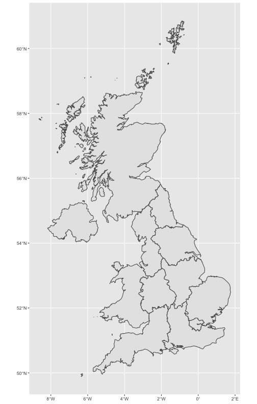<!-- --> ] --- .pull-left[ ```r t13_dt <- t13_dt %>% mutate(nuts118cd = case_when( region == "East" ~ "UKH", region == "East Midlands" ~ "UKF", region == "London" ~ "UKI", region == "North East" ~ "UKC", region == "North West" ~ "UKD", region == "Northern Ireland" ~ "UKN", region == "Scotland" ~ "UKM", region == "South East" ~ "UKJ", region == "South West" ~ "UKK", region == "Wales" ~ "UKL", region == "West Midlands" ~ "UKG", region == "Yorkshire and The Humber" ~ "UKE", TRUE ~ NA_character_ )) ``` * Rather than trying to match the different names/labels for the regions, it's better for use to use geographical codes, this makes sure both data.frames are talking about the same entities. * Using `dplyr::case_when` we can add the column `nuts11cd` to our data with codes assigned using conditional statements evaluating the `region` column. ] -- .pull-right[ ``` ## # A tibble: 12 x 3 ## region total nuts118cd ## <chr> <dbl> <chr> ## 1 East 21420 UKH ## 2 East Midlands 19910 UKF ## 3 London 89110 UKI ## 4 North East 29400 UKC ## 5 North West 54900 UKD ## 6 Northern Ireland 3690 UKN ## 7 Scotland 43930 UKM ## 8 South East 38610 UKJ ## 9 South West 40240 UKK ## 10 Wales 34110 UKL ## 11 West Midlands 28180 UKG ## 12 Yorkshire and The Humber 34090 UKE ``` ] --- .pull-left[ ```r map_dt <- sfdt %>% left_join(t13_dt, by = "nuts118cd") ``` * A key benefit of `{sf}` is that it easily integrates with the tidyverse methods. Here we have used `dplyr::left_join` to attach our data to the geographical data. ] .pull-right[ ``` ## Observations: 12 ## Variables: 12 ## $ objectid <int> 1, 2, 3, 4, 7, 5, 6, 8, 9, 10, 11, 12 ## $ nuts118cd <chr> "UKC", "UKD", "UKE", "UKF", "UKI", "UKG", "UKH", "UKJ"… ## $ nuts118nm <fct> North East (England), North West (England), Yorkshire … ## $ bng_e <int> 417313, 350015, 446903, 477660, 517516, 386294, 571074… ## $ bng_n <int> 600358, 506280, 448736, 322635, 178392, 295477, 263229… ## $ long <dbl> -1.728900, -2.772370, -1.287120, -0.849670, -0.308640,… ## $ lat <dbl> 55.29703, 54.44945, 53.93264, 52.79572, 51.49227, 52.5… ## $ st_areashape <dbl> 8609938893, 14182609113, 15432322860, 15658181358, 158… ## $ st_lengthshape <dbl> 657578.2, 1063052.7, 863264.1, 889656.3, 270855.1, 774… ## $ region <chr> "North East", "North West", "Yorkshire and The Humber"… ## $ total <dbl> 29400, 54900, 34090, 19910, 89110, 28180, 21420, 38610… ## $ geometry <MULTIPOLYGON [°]> MULTIPOLYGON (((-2.0344 55...., MULTIPOLY… ``` ] --- .pull-right[ ```r ggplot(map_dt) + geom_sf(aes(fill = total)) ``` * `geom_sf` allows us to plot `{sf}` objects in the same way as other data objects * Here we have mapped the `fill` aesthetic of the regions to the `total` variable ] -- .pull-left[ 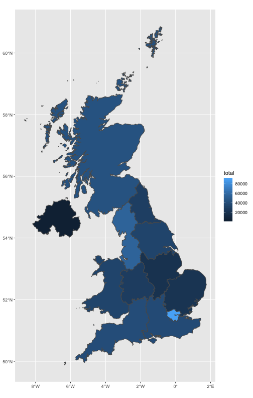<!-- --> ] --- .pull-right[ ```r theme_map <- function(...) { theme_void() + theme( legend.position = "none", ... ) } ``` * We can create a custom ggplot theme to remove the background features ] .pull-left[ <!-- --> ] --- .pull-right[ ```r ggplot(map_dt) + * geom_sf(aes(fill = total), colour = "white", size = 0.5) + * scale_fill_distiller(palette = "Oranges", direction = 1) + * theme_map() ``` * `geom_sf` allows us to plot `{sf}` objects in the same way as other data objects * Here we have mapped the `fill` aesthetic of the regions to the `total` variable * We have also applied a colour scale to change the map from the default blue ] .pull-left[ <!-- --> ] --- .pull-right[ ```r ggplot(map_dt) + geom_sf(aes(fill = total), colour = "white", size = 0.5) + * geom_sf_text(aes(label = total)) + scale_fill_distiller(palette = "Oranges", direction = 1) + theme_map() ``` * `geom_sf_text` allows us to add text labels using the coordinates from the sf object... let's use the the total column (our headcounts) ] .pull-left[ <!-- --> ] --- .pull-right[ ```r ggplot(map_dt) + geom_sf(aes(fill = total), colour = "white", size = 0.5) + * geom_sf_text(aes(label = scales::comma(total))) + scale_fill_distiller(palette = "Oranges", direction = 1) + theme_map() ``` * we can use `scales::comma` to format the number with a thousands separator ] .pull-left[ <!-- --> ] --- .pull-right[ ```r ggplot(map_dt) + geom_sf(aes(fill = total), colour = "white", size = 0.5) + * geom_sf_text(aes(label = paste(region, scales::comma(total), sep = ": ")) + scale_fill_distiller(palette = "Oranges", direction = 1) + theme_map() ``` * let's also add the region name to the label using `base::paste` ] .pull-left[ <!-- --> ] --- .pull-right[ ```r ggplot(map_dt) + geom_sf(aes(fill = total), colour = "white", size = 0.5) + geom_sf_text( * aes(label = * str_wrap(paste(region, scales::comma(total), sep = ": "), 12) * )) + scale_fill_distiller(palette = "Oranges", direction = 1) + theme_map() ``` * `stringr::str_wrap` provides a handy way of making strings wrap to a given length, in this case 12 characters ] .pull-left[ <!-- --> ] --- .pull-right[ ```r ggplot(map_dt) + geom_sf(aes(fill = total), colour = "white", size = 0.5) + geom_sf_text( aes(label = str_wrap(paste(region, scales::comma(total), sep = ": "), 12), * nudge_x = if_else(map_dt$nuts118cd=="UKI",1.25,0), * nudge_y = if_else(map_dt$nuts118cd=="UKJ",-0.25,0)) + scale_fill_distiller(palette = "Oranges", direction = 1) + theme_map() ``` * Finally, let's also adjust the x-position of London's label, and the y-position of the South East's label * We could alternatively create adjustment columns in our data table and add `nudge_x = x_adjust` to sf_text's `aes` mapping ] .pull-left[ <!-- --> ] --- .pull-right[ ```r ggplot(map_dt) + geom_sf(aes(fill = total), colour = "white", size = 0.5) + * geom_sf_label( aes(label = str_wrap(paste(region, scales::comma(total), sep = ": "), 12), nudge_x = if_else(map_dt$nuts118cd=="UKI",1.25,0), nudge_y = if_else(map_dt$nuts118cd=="UKJ",-0.25,0)) + scale_fill_distiller(palette = "Oranges", direction = 1) + theme_map() ``` * Switching to `geom_sf_label` provides a label background and border for the text ] .pull-left[ <!-- --> ] --- .pull-right[ ```r ggplot(map_dt) + geom_sf(aes(fill = total), colour = "white", size = 0.5) + geom_sf_label( aes(label = str_wrap(paste(region, scales::comma(total), sep = ": "), 12), nudge_x = if_else(map_dt$nuts118cd=="UKI",1.25,0), nudge_y = if_else(map_dt$nuts118cd=="UKJ",-0.25,0), * label.size = 0, alpha = 0.5) + scale_fill_distiller(palette = "Oranges", direction = 1) + theme_map() ``` * Finally, we can remove the border by setting `label.size` to 0, and adjust the background transparency via `alpha` ] .pull-left[ 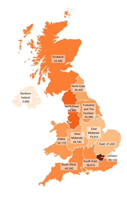<!-- --> ]